My Blog List

Friday, May 13, 2011

Admixture clusters, Mclust and populations concordance

First Excel spreadsheet includes 3 sheets for different Admixture runs (K=4),(K=7),(K=8).


Second Excel features additional statistic data:
1) Population concordance ratio (read more about this test in Dienekes' blog) - the row represents a test in which pairs of individuals from one populations were compared against individuals from the population of each column;
the column represents inividuals from same populations used as an "outgroup" for comparison against pairs of individuals from each row.

2) Mclust - using the Mclust package one can check if ADMIXTURE program correctly identify the clusters

3) K=8 for project's populations and members

IBS similarity matrix in R

Distributing IBS similiarity matrix as R data object becomes a good practice in other BGA projects. It is our turn to share IBS R data with project's members.

Please feel free to download R data file here.

The instructions assume that you have already got R installed:
1) In R console, type closest("ID"), where ID is a member's ID in project.
2) The default number of "neighbours" is 20, but you can change it by specifing the second argument, for example -closest ("V158",50).
3) Have fun.

Monday, May 9, 2011

IBD sharing

A couple of weeks ago i ran on my dataset ( 160 samples) a pairwise segmential IBD sharing analysis (in PLINK software). The analysis aimed at calculating genome-wide IBD given IBS information, as long as a large number of  independent, high quality SNPs  (c.300 000) were available pruning from the dataset SNPs below given MID,MAF and LD thresholds (the segmental sharing analysis requires approximately independent SNPs (i.e. linkage equilibrium) in a homogenous sample of unrealted individuals).

I followed the strategy suggested by the creators of PLINK software:

plink --bfile mydata2 --mind 1 --geno 0.01 --maf 0.05 --make-bed --out mydata3
followed by
plink --bfile mydata3 --indep-pairwise 100 25 0.2
followed by
plink --bfile mydata3 --extract plink.prune.in --make-bed --out mydata4 
 
I also removed a couple of relatives, since the focus of this analysis is to look for extended haplotypes shared between distantly related individuals: having very closely related individuals  will likely swamp the results of the analysis.

Here are results of PLINK analysis (in Excel format with more than 400 000 rows, so i can not upload it to Google Docs) (download link).


As I was expecting, the strongest  evidence of IBD sharing  was detected on Chr.6. Although the total number of pairwise shared segments (175) appears to be proportional to the length of chromosome 6, the average number of shared is about 2-3 times larger in comparisions to IBD segments on other chromosomes. Also the intersection of chromosome 6 shared segments produces apparent clusters.The detected preponderance of segmental IBD sharing on chromosome 6 is obviously explained by some well-known properties of Chr6 genomic areas. It is a well-known fact that human Chr.6 has one of the highest genotyping rate (SNPs per kbp), and the most of those SNPs are in very strong linkage (it also means that the default PLINK strategy for obtaining the set of SNPs in linkage equilibrium simply won't work for Chr 6).
Chromosome 6 also includes the human leukocyte antigen system (HLA) is the name of the major histocompatibility complex (MHC) in humans. The super locus contains a large number of genes related to immune system function in humans. This group of genes resides on chromosome 6, and encodes cell-surface antigen-presenting proteins and many other genes. The recent studies in medical genetics have revealed  the large level of IBD sharing in HLA, which is indicative of strong natural selection that affects (otherwise) discrete Poisson-like distribution of  IBD sharing probabilities.This particular property of IBD sharing in HLA region has been discussed in paper "Natural Selection and the Distribution of Identity-by-Descent in the Human Genome":

The largest excess of IBD sharing is in the HLA region on chromosome 6, where the mean posterior probability of IBD sharing within the CEPH individuals is about 0.06. The inferred IBD tracts on the entire chromosome are plotted in Figure S7A and the inferred tracts in the HLA region are plotted in Figure S7B. In total we infer 312 IBD tracts in the HLA region. The length distribution for these tracts is seen in Figure S7C. The length of most of the tracts are in the range of 0.5–7 Mb long in physical distances, but in genetic distances they are only 0.5–3.5 cM long (not shown). These tracts contain 30–309 SNPs; however, all SNPs contribute information to the inference of the tracts. Three of the tracts are exceptionally long (not shown in the length distribution). They belong to two unreported avuncular pairs and a sib pair present in the data. Excluding these pairs of individuals has little or no impact on the size of the overall signal (not shown).

The HLA region has some extreme recombination patterns and it has some of the highest amounts of LD found in the genome. In addition, it is a region that is difficult to genotype accurately because of the high degree of duplicated genes and structural variants. We therefore performed an additional test to validate the inferred IBD tracts. A subset of the CEPH sample consisting of 56 individuals overlaps with the original HapMap population. These individuals have been extensively genotyped using various genotyping platforms (International Hapmap Consortium 2007) with extra genotyping in the HLA region (De Bakker et al. 2006). Of the more than 10,000 SNPs available in the HapMap phase 2 database for this region we used only a small subset for our inference. This provided us the opportunity to validate our inferred IBD tracts using the additional data. If an inferred tract for a pair of individuals is truly an IBD tract then those two individuals should have at least one allele in common for all SNPs within a tract. If the two individuals do not share an allele identical-by-state (IBS) then the SNP is not compatible with the IBD tract. In Figure S8 we show the percentage of SNPs from the HapMap phase 2 genotyping data in each of the inferred tracts that do not share at least one allele IBS (incompatible). Of the 105 tracts inferred for the subset of individuals, only 4 have more than 0.5% (the genotyping error rate we used throughout this study) of the SNPs with an incompatibility in the HapMap phase 2 data. The vast majority of tracts have less than 0.1%. In contrast, if we randomly permute the individuals, we see that most of the tracts have between 1% and 10% pairwise incompatible genotypes. Thus the IBD region inferences within the HLA region are compatible, not only with the SNPs used for inferring the IBD tracts, but with all the available phase 2 HapMap SNPs in this region. This shows that the IBD tracts are not incorrectly inferred due to possible confounding factors, such as remaining LD, but are indeed real. Because the HLA region is hard to genotype we also examined the region for additional deviations from Hardy–Weinberg equilibrium. Using a Mann–Whitney test we found no difference in the distribution P-values between the HLA region and other parts of the genome. Finally, if IBD tracts were erroneously inferred due to genotyping error caused by hidden structural variants, we would expect to observe an excess of heterozygosity in individuals in IBD tracts compared to individuals not in IBD tracts in the same regions. We found no such excess in the HLA region (not shown).
The HLA region is also important for population genetics. The authors of paper "Linkage disequilibrium and age of HLA region SNPs in relation to classic HLA gene alleles within Europe"   discovered an important pattern of haploblock sharing:  haplotype blocks detected within HLA region, as well as classic HLA gene alleles and SNPs, were predictive of a northern versus southern European population membership (misclassification error rates ranged from 0 to 23%, depending on which independent population was used for prediction), indicating that this region may be a rich source of ancestry informative markers.  

It is believed now that HLA locuses belong to the set of ancestry informative markers that are used for inferring the genetic barriers on a worldwide scale.

In order to test the existence of  long extended IBD haplotypes,  i ran GERMLINE (an algorithm for discovering long shared segments of  (IBD) between pairs of individuals in a large population) on extracted subset of chromosome 6 "populations". GERMLINE takes as input genotype phased data for individuals (as well as an and generates a list of all pairwise segmental sharing. I used a pipeline for phasing PLINK format data with BEAGLE and processing in GERMLINE.

The analysis revealed explicit genetic signal of IBD sharing between Chuvashes and Finns. I haven't checked SNPs in detected haplotypes for ancestry information, but i assume that most of them are result of strong natural selection.


Wednesday, May 4, 2011

Troubles with StepPCO

Dienekes has brought my attention to StepPCO - a vanilla software used foe estimating the time of admixture events.

Genome Biology 2011, 12:R19 doi:10.1186/gb-2011-12-2-r19

Dating the age of admixture via wavelet transform analysis of genome-wide data

Irina Pugach et al.

Abstract

We describe a PCA-based genome scan approach to analyze genome-wide admixture structure, and introduce wavelet transform analysis as a method for estimating the time of admixture. We test the wavelet transform method with simulations and apply it to genome-wide SNP data from eight admixed human populations. The wavelet transform method offers better resolution than existing methods for dating admixture, and can be applied to either SNP or sequence data from humans or other species.

The software is written in R code and available online. For the past few days i was struggling with software troubles, trying to make this piece of code run on my computer. The basic problem here,however, is the lack of clear software documentation (there is a "readme" file in distro version of StePPCO, but it is not very helpful):

So, technically speaking, StepPCO workflow consists of 4 stages:
1)Calcuation of PCO object
source spco-wt.r into R
load the following required input files:
- genotype file: tab delimited file with genotypes for all the individuals (columns) and markers (rows); this file should be separate for each chromosome. Genotypes should be coded as 1 and -1 for the two homozygous alleles (AA and BB), 0 for the heterozygous (AB), use NA for missing data (My note: this genotype file could be easily constructed from TPED file format with some minor PERL and sed text parsing).

see example genotype file chr22 in Chr22.Rdata in this directory

- vector of physical positions of SNPs along a chromosome
see example PhysPos22 in Chr22.Rdata in this directory

- to generate plots you will need a color file, see example
colorfile.txt in this directory

EXAMPLE:
to calculate PC1 and PC2 using all individuals in our example genotype table, run

pco(chr22)->chr22.pco

In our example, genotypes are from 3 HAPMAP populations: columns 1:20
contain genotypes for ASW (individuals of African ancestry from the
Southwestern USA, known to have European admixture), columns 21:40
contain genotypes for CEU (individuals of European ancestry), and
columns 41:60 contain genotypes for Yoruban (YRI) individuals from
sub-Saharan Africa. To use only parental populations (CEU and YRI) for finding principal axes, and
and then to project admixed inds (ASW) onto it, run

pco(chr22, axis.who=colnames(chr22[,21:60]))->chr22.pco

to plot your results, run:
plot.pco(chr22.pco)

if you don't want to see individual labels for each sample, use:
plot.pco(chr22.pco, names="none")

2. Calculation of SPCO
Calculation of SPCO:
source spco-wt.r into R
the following input files are required:

- genotype file
see example genotype file chr22 in Chr22.Rdata in this directory

- vector of physical positions along a chromosome of all SNPs in the genotype file
see example PhysPos22 in Chr22.Rdata in this directory

- table of genetic distances (in cM) between all SNPs in the genotype
file
see example GenMap22 in Chr22.Rdata in this directory

To generate such GenMap file we downloaded genome-wide recombination
rates estimated as part of the HapMap project
(http://hapmap.ncbi.nlm.nih.gov/downloads/recombination/latest/rates/),
read the
http://hapmap.ncbi.nlm.nih.gov/downloads/recombination/latest/rates/genetic_map_chr22_b36.txt
into R, and interpolated genetic distances, using:

interpolate.genetic.map(PhysPos22, hapmap.table)->GenMap22

- to generate plots you will need a color file, see example
colorfile.txt in this directory

To run call:
spco(table,....)

EXAMPLE:
to calculate StepPCO for our example genotype table, using YRI and CEU
as parental populations, and "3 sigma" as a window method, run

spco(chr22, pco=chr22.pco, genetic.map=GenMap22, Nbins=1024, window.size="3 sigma",pop1=colnames(chr22[,21:40]),pop2=colnames(chr22[,41:60]),max.window.size=Inf)->spco.chr22

to plot results for a particular admixed individual
(e.g. "ASW_20126"), use:

plot.spco.stats(spco.chr22, who=colnames(chr22)[19], main=paste("SPCO: CEU, YRI and ",colnames(chr22)[19]," Chromosome 22", sep=""))
3.Wavelet transform
source spco-wt.r into R

calculated spco is required as input

EXAMPLE:
to run wavelet transform analysis for our example genotype table, first calculate spco and then use:

spco.wtstats(spco.chr22, threshold=0.1, maxlevel=5)->wtstats.chr22

to filter out noise and normalize:
for each level find a threshold amplitude, which is present in every individual whether admixed or not, remove everything below it as noise and recalculate "centers":

threshold.chr22<-vector() for (i in 1:5){max(wtstats.chr22$wt.summary[c(21:60),i],na.rm=TRUE)->threshold.chr22[i]}

for (i in 1:60){cutoff(wtstats.chr22$wt.summary[i,1:5],thr=threshold.chr22[1:5])->wtstats.chr22$wt.summary[i,1:5]}

for (i in 1:60){wtstats.chr22$wt.summary[i,"center"] <- sum(wtstats.chr22$wt.summary[i,1:5]*(1:5))/sum(wtstats.chr22$wt.summary[i,1:5])} to normalize subtract from each calculated "center" log2 of the length of chromosome in Morgans: wtstats.chr22$wt.summary[,"center"] <- (wtstats.chr22$wt.summary[,"center"]) - (log2(0.7366522))


4.Time of admixture estimate


Time of admixture estimates are based on comparison to the results obtained for simulated data. For instructions on how to run simulations see README.recsim file.


Despite all my efforts ito make this particular software run, i wasn't able to get past the second stage -SPCO calculation. I used a genotype file for Chr1, extracted from the transposed PLINK dataset of MDL project, a file with physical positions of snps and genetic map (with included genetic distances in cM). The first part - PCO caclulation -seemed to run smoothly, alhtough there are some problems with memory optimization, and i was able to make PCA plot from calculated PCO object (see plot attached below). In contrast to that, SPCO calculation, after running some 45-50 minutes, exited with series of marshalling errors. I have reported this bug to software's developpers and will be waiting for their instructions.


Tuesday, May 3, 2011

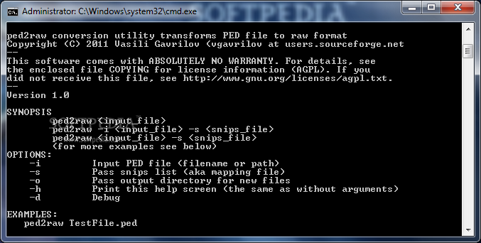
PED2RAW is now featured on Softpedia

PED2RAW is now featured on Softpedia. Congrats to Vasily Gavrilov.


Synopsis:

Convert PED genome file fast and easy.

ped2raw is a small, command prompt based application specially designed to help you convert PED genome file into RAW SNP format. Creates multiple files per PED file, i.e. 1 file per person and it offers support for big files.

Because it's command prompt based, don't expexct any fancy GUI to guide you through the conversion process. So, to convert PED files, take ped2rawfor a spin and check out its capabilities.

http://www.softpedia.com/get/Multimedia/Graphic/Graphic-Others/ped2raw.shtml


STRUCTURE (K=10, N=159) results


STRUCTURE (K=10, N=159, 7 CPU days) results


Grapho-analytical approach to the visualisation of IBD shared segments

I just wasted 2 past weeks thinking of new method for visualising the scope of IBD segments' "sharedness" between different populations in project. I, personally, consider PLINK-based inference of  overlapping IBD segments to be very useful for the project's purposes . PLINK has functions to detect specific segments shared between distantly- related individuals, for discovering long shared IBD segments, one can use GERMLINE algorithm.


As mentioned in PLINK's manual, the --segment option in PLINK command line generates a file plink.segment  which has the fields (one row represents one segment between two compared individuals):

FID1       Family ID of first individual
     IID1       Individual ID of first individual
     FID2       Family ID of second individual
     IID2       Individual ID of second individual
     PHE        Phenotype concordance: -1,0,1
     CHR        Chromosome code
     BP1        Start physical position of segment (bp)
     BP2        End physical position of segment (bp)
     SNP1       Start SNP of segment
     SNP2       End SNP of segment
     NSNP       Number of SNPs in this segment
     KB         Physical length of segment (kb)
To get an idea of how IBD segments file may look like, you may want to take a look at an example of  Plink segment file, which includes a list of estimated IBD sharing segments between MDL project participants (download link).

The first thing what came in my mind  when  i was tackling  IBD OVERLAP and INDIV file formats, was to read IBD sharing data as graph objects. At least, i have not figured out a better solution and grapho-analytical approach is very straightforward. Suppose, you want to read shared segments file in R, assuming that graphs of sharedness is undirected. Then, R-routine for reading in the file and converting to an igraph object is very simple:

library(igraph)  
segments <- read.csv("IBD.shared.segments", header = F)
g <- graph.data.frame(seg, directed = F)
ecount(g)
//returns number of vertices
vcount(g)
//returns number of edges
Given a graph object (read in and transformed from  PLINK segment file format) and a set of graph manipulation rules, one can basically do with graphs whatever he or she intends to do.  For instance, one can calculate the largest “clique” of graph and create  a new graph of that largest clique. A clique is a maximally-connected subgraph in which every vertex connects to every other vertex:

lc <- largest.cliques(g)
g.lc <- subgraph(g, lc[[1]])

One can also assign uniformly random weights to the edges and set the color edge attribute to “red” for edges with high weight, and  find the shortest path between two nodes of graph, etc.

More details about igraph object on Igraph's homepage.


Please consider the real-life example of graph, representing the amount of sharedness between project participants. What can we learn from the graphical representation of project's "communities" based on the amount of IBD sharedness? In our particular case we can easily identify the patterns of "IBD sharedness" within and between populations. For example, there are two "IBD communities" in Finnish "population sample" in our project (black circles on the graph). These two enigmatic "communities" appear to be "things in themselves" being focused on two sharing "midpoints" in Finnish sample (V151;V156), while V151 and V156 appear to be only Finns linked by means of IBD segment sharing to North_Russians, and, to lesser extent, Balto-Slavic cluster.

That looks pretty cool.