Behind the Curtains: MDLP World 22 showcase

Preliminary remarks

As you all may know, the MDLP  blog hasn't been updated since February 2012.

Half of year ago i promised myself that i would stop writing new posts on the MDLP blog before i'll finally get my scientific report on blog written.  Since I had to prioritize the completion of a scientific paper over the routine of blog posting,I was unable to continue updating the blog on a regular basis due to a lack of time, and had to make a change in how I conducted my research. So i decided to abstain from posting on the MDLP blog for a couple of month, being focused on more important matters. Despite of all limitations, i kept  working secretly on the MDLP project, collecting necessary data and performing different 'genomic' experiments in order to achieve my final goal (publishing of paper).  The results of secret experiments with new genomic samples and tools eventually leaked to the curious public, spawning immense interest in my project. After releasing a new version of my own modification of DIYDodecad calculator on Gedmatch.com, i was literally flooded by emails from Gedmatch.com users asking me  questions they wanted me to answer.

I understood the strategical mistake of releasing poorly documented data/analysis on Internet  and felt obliged  to explain details. Obviously, i will start new series of  the blog posts by covering the project feature the people most interested in, i.e the MDLP World22 calculator.
 

The population dataset of MDLP World22 calculator.

The reference population dataset of the calculator was assembled in PLINK by intersecting and thinning the samples from different data sources: HapMap 3 (the filtered dataset CEU,YRI,JPT,CHB), 1000genomes, Rasmussen et al. (2010),  HGDP (Stanford) (all populations),  Metspalu et al. (2011),Yunusbayev et al. (2011), Chaubey et al. (2010) etc. Furthermore i handpicked random 10 individuals from each European country panel in POPRES dataset, or the maximum number of individuals available otherwise, to select the POPRES European individuals to be included in our study. Finally, in order to evaluate the correlation between the modern and the ancient genetic diversity, i have also included ancient DNA genomic samples of Ötzi,(Keller et al.(2012)) Swedish Neolithic samples Gök4, Ajv52, Ajv70, Ire8, Ste7 (Skoglund et al. (2012)) and 2 La Braña individuals from the Mesolithic sites of the Iberian Peninsula (Sánchez-Quinto et al.(2012)). Then i added 90 samples of individuals-participants of our MDLP project.  After merging the aforementioned datasets and thinning the SNP set with PLINK command to exclude SNPs with missing rates greater than 1% and minor alleles, i filtered out duplicates, the individuals with high pairwise IBD-sharing  (estimated in Plink as as the average fraction of alleles shared between two individuals over all loci) and the individuals with kinship coefficient suggesting relatedness (kinship coefficients were estimated in KING software). Also i had to filter out individuals with more more tham 3 standard deviations from the population averages. Since kinship coefficient is robustly estimated by HWE (Hary-Weinberg expectations) among SNPs with the same underlying allele frequencies, SNPs showing strong deviation (p < 5.5 x10⁻⁸) from Hardy-Weinberg expectations were removed from the merged and filtered dataset. After that I filtered to keep the list of common SNPs present in Illumina/Affymetrix chips and performed  linkage disequilibrium based pruning using a window size of 50, a step of 5 and r^2 threshold of 0.3.

This complex sequence of consequent operations with the initial reference and project datasets yielded a final dataset which included 80751 SNPs  in 2516 individuals from 225 populations.


ADMIXTURE analysis

 As always, the final dataset in PLINK linked format was further processed in ADMIXTURE software. Sketching the plan for the design of ADMIXTURE test,  i had to face the difficult problem: as it has been shown in (Patterson et al.2006) the number of markers needed to resolve populations in ADMIXTURE analysis is inversely proportional to the genetic distance (Fst ) betweeen the populations. According to ADMIXTURE best practice, it is believed that 10,000 markers  are suffice to perform GWAS correction for continentally separated populations (for example, African, Asian, and European populations FST > .05) while more like 100,000 markers are necessary when the populations are within a continent (Europe, for instance, FST < 0.01).

To increase the accuracy of ADMIXTURE results i decided to use a method proposed by  Dienekes' for converting allele frequencies into 'synthetic individuals'(see also Zack's example). The idea is fairly simple: run an unsupervised ADMIXTURE analysis once to generate allele frequencies for your K ancestral components; then generate zombie populations using these allele frequencies; whenever you want to estimate admixture proportions in new samples run supervised ADMIXTURE analysis using the zombie populations.  Like any genome blogger engaged in the task of evaluating admixtures in samples, i must grapple with obvious question of the reliability of this approach.  Although i am aware of  methodological controversies in using simulated individuals, i would rather concur with Dienekes who considered "synthetic individuals" the best abstract proxies for the ancient ancestral populations. But my purpose is served if i can use the approach used by Dienekes and Zack to obtain meaningful results. To begin with, i routinely ran unsupervised ADMIXTURE  K=22 analysis (assuming 22 ancestral populations) which yielded the admixture proportions of individuals from these K populations, as well as the allele frequencies for all SNPs for each of 22 ancestral populations (below are conventional names for each of inferred components in order of appearance):

Pygmy
West-Asian
North-European-Mesolithic
Tibetan
Mesomerican
Arctic-Amerind
South-America_Amerind
Indian
North-Siberean
Atlantic_Mediterranean_Neolithic
Samoedic
Proto-Indo-Iranian
East-Siberean
North-East-European
South-African
North-Amerind
Sub-Saharian
East-South-Asian
Near_East
Melanesian
Paleo-Siberean
Austronesian

Therefore i took the allele frequencies which were computed earlier in unsupervised Admixture K=22 for the merged dataset, pooled them into PLINK and generated 10 "synthetic individuals per ancestral component) using PLINK command --simulate.  When the simulation had been  finished, i visualized the distance between simulated individuals using multi-dimensional scaling:



 

As a next step,i included simulated individuals you have as part of a new reference population (including 220 simulated individuals in 22 simulated populations).Then, I ran ADMIXTURE anew, this time in “supervised” mode for K = 22 (with simulated individuals being 'reference' individuals). The Admixture K=22 converged in 31 iterations (37773.1 sec) with final loglikelihood:-188032005.430318 (below are Fst divergences between estimated 'ancestral' populations):

The Fst distance/divergence matrix was used for inferring a most probable NJ-based topology of component distance tree (outgroup: South-African):

 The individual 'supervised' ADMIXTURE  results (in Excel spreadsheet) for the project participants have been uploaded to GoogleDocs (please note that the average results for reference populations is also available on special request).

MDLP World22 DIYcalculator

The output files of Admixture K=22 supervised run (average values of admixture coefficients in reference populations and FsT values)  were used for designing a new version of  the MDLP DIYcalculator, which is better known by its codename "World22" (online version is available in AdMix-Utilities section of Gedmatch under MDLP project). MDLP DIYcalculator itself is based on the code of Dodecad DIY calculator (c)ourtesy of Dienekes Pontikos and was developed as part of the Dodecad Ancestry Project. In its Gedmatch implementation MDLP 'World22' DIYcalculator is paired by MDLP 'World22' Oracle, also based on Dienekes' and Zack's code (Harappa/DodecadOracle). The 'Oracle' is designed to find in a single population mode your closest (closest in terms of similarity) population from MDLP ''Word22' admixture results. In a mixed mode, Oracle considers all pairs of populations, and for each one of them calculates the minimum Fst-weighted distance to the sample in consideration, and the admixture proportions that produce it.

Please notice: 'ancestral' populations (i.e 'simulated populations' from the previous step - see above) are labeled in Oracle results as (anc), while the 'real world' modern and ancient populations are marked as "derived".

If you have troubles with understanding/interpreting the results of Oracle and DIYcalculcator, please consult the corresponding topics on Dodecad and HarappaWorld blogs. It is not of avail to repeat in this blog everything they wrote in their own blogs.

What the heck are MDLP Word-22 components?

 One of those questions that i usually keep getting in emails is what do the various reference populations and ancestral components for my World K=12 and World-22 analyses mean. I've already provided hints to the answer  earlier, but - as old Chinese proverb says - one picture is worth ten thousand words. That's why i decided to display the admixture coefficients spatially on the globe surface. Following Francois Olivier, who proposed to use the graphical library of the statistical software R to display  spatial interpolates of the admixture coefficients (Q matrix) in two dimensions (where spatial coordinates are recorded as longitude and latitude), i created  2 contour maps per component.

Pygmy (modal in Biaka and Mbuti population)

West-Asian (bimodal component with peaks in Caucasian populations and south-western part of Iran, equal to Dienekes' Caucasian/Gedrosia component) 

 North-European-Mesolithic (local component with peaks in European Mesolithic samples of La_Brana and  modern North-European Saami population).

 Tibetan (Indo-Burmese) component (Himalay, Tibet)

Mesomerican (major genetic component in Native Americans from Mesoamerica)

North-Amerind (the 'native' component in North American Natives)

South-Amerind (the 'native' component in South American Natives)

  Atlantic-Mediterranean-Neolithic (the main genetic component  in Western and South-Western Europe)

  The rest contour maps for all components could be downloaded here.






   

Rising from The Ruins

The MDLP blog is back online again.

Please support this blog by donating to PayPal account of the project

Comparing fineSTRUCTURE clustering to Mclust clusterings

The first weeks of 2012 years marked a milestone in  BGA blogging paradigm , introducing substantial shift of methodologies.

First of all, Eurogenes blog has applied recently published Chromopainter tools to its intra-North Euro cluster analysis (with more than 400 samples and 270K SNPs, in linkage mode, and 200K burn-ins and iterations).

Dodecad Project  has also improved its  Cluster Galore method  to be  used with linked haplotype data (this refined method is , however, designed, to work not wiyj fineSTRUCTURE, but with different software fastIBD).

Although both methods are different in technical performance and design, they still strive for the same goal of inferring the population structure. This type of structure inference consists of two parts: deriving a matrix of relationships between sampled individuals and clustering these relationships.  As was noted by Dan Lawson , given a distance-like matrix such as the number of SNPs IBS or the ChromoPainter coancestry matrix, it is possible to apply a wide variety of clustering algorithms. 

Still fineSTRUCTURE has two advantages. Firstly, because fineSTRUCTURE performs MCMC it is less likely to get stuck in local optima than computationally cheaper methods that climb gradients. Secondly, and most importantly, (when used correctly) fineSTRUCTURE is well calibrated as it has no unknown and hard to estimate tuning parameters. 

Experiment

In order to evaluate the performance of different clustering methods on a real-world dataset, i used sampled individuals from my project. To make this test experiment even harder, i've applied Chromopainter's algorithm (*linkage mode) to a homogenous uniform subset of very similar Baltic Populations: Lithuanians, Belorussians, Ukrainians (90  samples plus a couple of reference Belorussian, Lithuanian and Ukrainian samples with 90K SNPs).  The same dataset was used in Shellfish to carry out a  principal component analysis of genome-wide SNP data, and in PLINK MDS-calculations. Obtained PCA and MDS data was subsequently analyzed using the general-purpose clustering software Mclust.

I ran Chromopainter's algorithm separately on each of 22 chromosomes, the output files were merged into one single file. Then i applied fineSTRUCTURE's MCMC algorithm to infer the population structure, PCA components and cluster trees. Below are plots showing individual co-ancestry matrix, individual and population agglomerate plots and PCA plots.

It appears that fineSTRUCTURE inferred 5 clusters (starting with smallest): (1) Ashkenazi, (2) individuals of West-European origin with (moderate to minor) East-European "admixture" (3) individuals from East-Europe and (4) Lithuanians, (5) the biggest cluster including Poles, Belorusians, Russians and Ukrainians.
For our project's particular purposes, it is important to note that such a clear split between Belorussians and Lithuanians is introduced for the first time. Although the innuendo of this division could be inferred from our earlier experiments, the statistical signal of separation was weak  enough to be ignored, because (as it is shown on the plot below) some regions of the plots are highly uncertain.

The cluster assignments (fineStructure) for project's individuals can be seen here.
 I have also published corresponding cluster assignments by Mclust (PLINK+MClust and Shellfish+MClust).  Direct agreement between these two latter solutions: 0 of 4 pairs, iterations for permutation matching: 24, cases in matched pairs: 34.58 %

     2  3  1  4
  1  0  2  3  0
  2  2  8  1  3
  3 13 11 16 18
  4  4  4  9 13














 

Last posting in the year 2011

Earlier this month I experimented with Chromopainter and fineSTUCTURE software. For the sake of comparision with ADMIXTURE/LAMP results, i used PLINK linkage file with previously extracted SNPs on Chr.6. The PLINK file included thinned set of LD-pruned SNPs (9155 SNPs in total). I also limited the dataset to include the projectäs participants only. I streamlined the phasing of this dataset by using Gusev's phasing_pipeline (which is indispensable for conversion between PLINK and BEAGLE format, and phasing genotypes with BEAGLE).

After that i deployed plink2chromopainter.pl, a conversion script for going from PLINK linkage-style PED and MAP files to ChromoPainters PHASE and MAP files. The converted MAP file was merged with HapMap's pre-compiled recombination file for Chr.6 (in order to accomplish this task i used a simple buggy but efficient AWK script). This trick allowed me to avoid/skip the painstaking exercise in UNLINKED model of Chromopainter .

As a next step, i changed default -k parameter to 200 (to give approximately 200 random samples to estimate the local variance). It is important to mention, that Chromopainter could be run in two modes: "donor mode" (which assumes the prior existence of "donor" and "recipient" haplotypic populations) and "all against all" mode. I we used the latter approach in which a single haplotype within an individual is reconstructed using the haplotypes from all other individuals in the sample as potential donors. This process is repeated for every haplotype in turn, so every individual is ultimately reconstructed in terms of all the other individuals, i.e every individual in my sample is conditioned on all the other individual.

It took me approximately 1,45 hours to finish Chromopainter's job. After that in combined Chromopainter output files, creating the file "MDLP.Chr6.chunkcounts.out", which is the coancestry matrix that fineSTRUCTURE requires as input.

After that i fed fineSTRUCTURE with required input (the coancestry matrix) and let fineSTRUCTURE to find a correct number of sample's "splits" (clusters). Surprisingly, even in such a limited (LD-prunned and tiny) dataset of SNPs, fineSTRUCTURE was able to detect four population-like (2 East-European, 1 West-European and outliers) clusters. In comparision, ADMIXTURE had some troubles with fleshing out sample's K-clusters, when i ran it on both phased and unphased version of the same Chr6. dataset (you can see them in this Excel spreadsheet).

From what i gather, author's claim holds water: fineSTRUCTURE indeed outperform ADMIXTURE/STRUCTURE approaches: "We next turn to our fineSTRUCTURE model-based analysis, again considering the unlinked coancestry matrix even though strong and variable LD exists in the dataset. We first compared performance of our unlinked model to the popular ADMIXTURE [15] software (Figure 3B and D, details in Section S8). Encouragingly, as the number of 5Mb regions increased from 5 to 200 we saw a monotonic performance increase for the no-linkage model, separating all groups with 200 markers. Further, our approach outperformed ADMIXTURE, with the ADMIXTURE performance levelling at around 60% correlation with the truth. In practice, we observed ADMIXTURE successfully splitting groups A, B and C and mostly splitting C1 and C2, but not B1 and B2, as detailed in Figures S6-11. ADMIXTURE performs inference under a model where markers are treated as unlinked, and where individuals may have genomes made up of mixtures of inferred source populations, while our simulation incorporated drift between populations, but not admixture. To examine whether violations of both these modelling assumptions explain the different results, we simulated a new dataset with the same underlying population structure of 5 populations as before, but no linkage (i.e. independence) between markers within each population. We analysed these data with STRUCTURE, which uses a similar underlying model to that of ADMIXTURE, but includes a no-admixture model (Section S7). For small datasets, STRUCTURE slightly improved performance relative to our unlinked fineSTRUCTURE model, but for larger SNP numbers, fineSTRUCTURE was able to identify all population splits (K = 5) while again, STRUCTURE was able to split only populations A, B and C (K = 3). Thus, even when LD information is not used (or even present), fineSTRUCTURE can offer advantages in some settings over these existing approaches."

With this gist of fineSTRUCTURE methodology, is is now safe to conclude that the combined set of all 22 chromosome, the linkage model can do even better. 

The painting process gives three square matrices of size NxN (N=number of individuals): 1) the frequency individuals copy chunks from each other, 2) the average length of those chunks, and 3) the mutation rate. These contain different aspects of the ancestry history, and almost completely summarize population ancestry.

The origin of some individual haplotypes could be ascertained using more comprehensive GERMLINe matching algorithm. Indeed, after applying GERMLINE algorithm to BEAGLE-phased chromosomes (1..22), i can see that the pairwise matches in haplotypes located far away from the chromosomal centromere and telomeres, tend to cluster into "ethnic" groups. However, haplotypes which are observed near centromere, are rather omnipresent - as would be expected if these regions had low rates of recombination because of proximity to centromeres.  The IBD segments detected by GERMLINE are listed (per chromosome) below:

Chromosome12

Chromosome11

Chromosome13

Chromosome14

Chromosome19

Chromosome15

Chromosome20

Chromosome9

Chromosome8

Chromosome18

Chromosome21

Chromosome21

Chromosome 6

Chromosome 7

Chromosome 17

Chromosome 16

Chromosome 10

Chromosome 22

Chromosome 5

With the scope on xMHC (see our previous posting),Of special interest here are, perhaps, haplotype matches on Chromosome 6, which match the pattern of massive extensive sharing of linked SNPs in the region of xMHC  - Chrom6-cM

Experimental test: inferring HLA (haplo)types from DNA nucleotide sequences using HLA*IMP framework

Molecular differences between HLA alleles vary up to 57 nucleotides within the peptide binding coding region of human Major Histocompatibility Complex (MHC) genes, but it is still unclear whether this variation results from a stochastic process or from selective constraints related to functional differences among HLA molecules. Although HLA alleles are generally treated as equidistant molecular units in population genetic studies, DNA sequence diversity among populations is also crucial to interpret the observed HLA polymorphism (Buhler S, Sanchez-Mazas A, 2011 HLA DNA Sequence Variation among Human Populations: Molecular Signatures of Demographic and Selective Events. PLoS ONE 6(2): e14643. doi:10.1371/journal.pone.0014643).

Traditionally, serology has been used for HLA typing for many decades; however, serological typing of histocompatibility class II molecules depends on the adequate expression of these molecules on the surface of B lymphocytes, the availability of viable cells and a complete set of antisera. However, the application of molecular methods (RFLP, PCR, SSO etc.) to HLA typing has led to the situation whereby nearly every laboratory performs some DNA typing for the detection of HLA alleles.

Why HLA loci are so important?

 HLA loci present the highest degree of polymorphism of all human genetic systems. Prior knowledge of the extent of diversity is essential in the development and selection of molecular typing methods. Reliable allele frequencies are also important in allogeneic unrelated hematopoietic stem cell transplantation to determine the likelihood of finding closely HLA matched donors for each patient.The genetic diversity of the HLA loci is responsible for the efficiency of the immune system in eliminating cells carrying foreign antigens. There is a need to develop a measure of this genetic diversity in order to assess how different populations are equipped to respond to foreign-antigen exposure, and to evaluate the contribution of each HLA locus.

The HLA system has been extensively studied from an evolutionary perspective. The region contains a number of closely linked genes whose products control a variety of functions concerned with the regulation of immune responses. In addition, the genetic predisposition to over 40 diseases maps to this region. A number of observations indicate that strong selection is acting on the HLA region, including its extensive polymorphism with very even allele frequencies, the preferential occurrence of high levels of variability at positions critical to antigen recognition, the great age of alleles and the patterns of linkage disequilibrium among loci. The form of the selection is unknown. Although balancing selection is a strong candidate, it seems unlikely that only one selective mechanism is operating in this complex multigene family region. Mutation, recombination and gene conversion all contribute to the generation of HLA variability. The apparent great age of many HLA alleles revealed by phylogenetic analysis suggests that the absolute rate of production of new variants is not high. Detailed studies of population and evolutionary features of the HLA region are necessary for an informed discussion of the evolution of disease predisposing genes and epitopes, and of complex multigene families (Thomson G.HLA population genetics.1991 Jun;5(2):247-60.)

Nomenclature of HLA Alleles

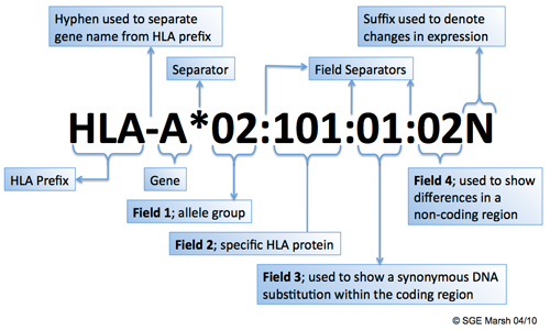
Each HLA allele name has a unique number corresponding to up to four sets of digits separated by colons. The length of the allele designation is dependant on the sequence of the allele and that of its nearest relative. All alleles receive at least a four digit name, which corresponds to the first two sets of digits, longer names are only assigned when necessary.The digits before the first colon describe the type, which often corresponds to the serological antigen carried by an allotype. The next set of digits are used to list the subtypes, numbers being assigned in the order in which DNA sequences have been determined. Alleles whose numbers differ in the two sets of digits must differ in one or more nucleotide substitutions that change the amino acid sequence of the encoded protein. Alleles that differ only by synonymous nucleotide substitutions (also called silent or non-coding substitutions) within the coding sequence are distinguished by the use of the third set of digits. Alleles that only differ by sequence polymorphisms in the introns or in the 5' or 3' untranslated regions that flank the exons and introns are distinguished by the use of the fourth set of digits (further information: http://hla.alleles.org/nomenclature/naming.html).

Example

HLA-A    identifies HLA A locus
HLA-A1 serologically defined antigen
HLA-A* asterisk denotes HLA alleles defined by molecular methods
HLA-A*01 2 digit resolution denotes a group of alleles corresponds usually to serological group – low resolution
HLA-A*0101 4 digit resolution – sequence variation between alleles results in amino acid substitutions
HLA-A010101 6 digit resolution – non coding variation: sequence changes synonymous no amino acid substitution



HLA types and linked SNPs

 Still, classical HLA alleles (e.g. HLA-, HLA-B, etc.) are tricky to analyze with chip technology employed in popular commercial personal genomic services (23andme, FTDNA's Family Finder and deCODEme) , because analysis is a complex process, requiring a large number of multiplex PCR reactions to obtain a patient's full genotype. That is why classical HLA typing methods are often imparctical for large-scale studies.

Fortunately for us , Wellcome Trust Centre for Human Genetics described a method for imputing classical alleles from linked SNP genotype data, implemented in the imputation framework (HLA*IMP) (Alexander Dilthey, Loukas Moutsianas, Stephen Leslie, and Gil McVean. HLA*IMP – an integrated framework for imputing classical HLA alleles from SNP genotypes Bioinformatics btr061 first published online February 7, 2011 doi:10.1093/bioinformatics/btr061).

HLA*IMP  imputes HLA type information based on SNP genotype, using methods of iterative model building to select a set of informative SNPs  for particular supported genotyping chips (AffyMetrix 500K, AffyMetrix 900K, Illumina 300K, Illumina 550K,Illumina 650K, Illumina 1M). Thus, HLA*IMP enables researchers to perform classical HLA allele imputation from genotype data collected from several available genome-wide SNP sets through reference to a reference data set of over 2,500 samples of European ancestry with dense SNP data and classical HLA allele types. This reference set includes:

• The 1958 Birth Cohort  typed both on the Illumina 1.2M and Affymetrix Genome-Wide Human SNP Array 6.0 chips (TheWellcome Trust Case Control Consortium, 2007) - 2420 genotype samples x 7733 SNP  in the extended HLA region.
• The HapMap CEU samples (The International HapMap Consortium, 2007) and CEPH CEU+ additional samples (de Bakker et al., 2006)    - 92 samples x 7733 BC58-overlapping SNPs)

SNP haplotypes for the 1958BC and CEU+ samples were phased using IMPUTE v2  using the trio-phased HapMap samples as a reference dataset. Classically typed HLA genotypes were then phased into SNP haplotypes by using PHASE (Stephens and Scheet, 2005) applying standard settings for multiallelic loci. The combined reference dataset consists of 5024 haplotypes with data on 7733 SNPs in the HLA region. This splits up into 2474 (HLA-A), 3090 (HLA-B), 2022 (HLA-C), 175 (HLA-DQA1), 2629 (HLA-DQB1), 2665 (HLA-DRB1) locus-specific haplotypes which are used for inference.

The experiment with MDLP dataset

Motivation:

As i previously mentioned in my blog (re: Chromosome 6), 23andme's RelativeFinder and AncestryFinder revealed (among my results) a cluster of a prominent number of HIR-matches (315), positioned in the exactly the same subregion of HLA-MHC domain on Chr.6 (21Mb-38Mb). This remarkable group of matches constitutes almost a half of my total AF/RF matches (315/720 or 43,75%).

Earlier i suggested that such a preponderance of HIR-matches to HLA region is indicative of case of sharing the same extended HLA haplotype. Until recently, my suggestion rested solely on my intiution.  Then, i found solution to HLA*IMP challenges and so far, i've managed to make HLA*IMP work with 23andme genotyper (Illumina Omnio Express) call raw data.

For my test, i needed to make sure that my data meets the following requirements:

• SNPs must be from the xMHC region (chromosome 6) 
• European ancestry of the typed individuals 
• sufficient quality and typed SNP density in the HLA region to enable reliable phasing
• since HLA*IMP doesn't provide a direct support for 23andme's chips and i was using the combined set of genotypes from 23andme's chipset v2 and chipset v3, i've choosed "a downgraded" version of Illumina genotyping platform (Illumina 300K)

In order to my initial assumption of HLA haplotype sharing i selected 7 participants from my project (including 4 individuals without  HIR-sharing on Chromosome 6 (not detected by 23andme's AF)  me, my mother and an individual, who has a HIR-match with me and my mother in xMHC region). I  converted 23andme's raw data of the project's participants into Plink format,  merged the files into one dataset and extracted SNPs on Chromosome 6 using Plink command --chr 6. After that, i converted the genotype data from Plink format to HLA*IMP input data format. As a next step, i carried out quality control  on the genotype data, removing SNPs and individuals with too much missing data and aligning complementary SNPs to the HapMap reference strand. Finally, i phased  included genotypes to obtain haplotype data. Note: each individual was anonymized by substituting project's ID with prefix N.

The haplotype data was uploaded to HLA*IMP back-end web service    for imputing HLA types.

The imputed HLA types look as follows (each individual is represented by 2 HLA haplotypes in HLA-A:HLA-B:HLA-C:HLA-DQA:HLA-DQB:HLA-DRB format)

IndividualID	Chromosome	HLAA	HLAB	HLAC	HLADQA	HLADQB	HLADRB
N1	1	101	801	701	501	201	301
N1	2	2601	2705	102	101	501	101
N6	1	3101	801	701	501	201	301
N6	2	201	1501	304	501	201	301
N3	1	6801	1501	102	101	501	101
N3	2	2301	5201	501	101	501	101
N2	1	101	801	701	501	201	301
N2	2	2601	3801	1203	102	602	1501
N5	1	301	1501	304	501	302	401
N5	2	205	5001	602	501	202	701
N7	1	101	801	701	501	301	1101
N7	2	101	1501	303	103	604	1301
N4	1	301	702	702	401	402	801
N4	2	2402	4002	202	501	301	1101

The haplotypes should be read as  follows (for example, in case of N1): HLA A*0101 : Cw*0701 : B*0801 : DRB1*0301 : DQA1*0501 : DQB1*0201. 

From the table posted above, one can easily mention a matching pattern between  N1, N2 and N7, as they share the similiar haplotype.  As a matter of fact N1 (ny mother), N2 (me) and N7 share HIR-segment (matching DNA segment equal to or greater than seven Centimorgans (abbreviated as cMs) on one segment with 700 or more SNPs), found by RelativeFinder service at 23andme.

Thus, it is safe to conclude that the imputation was accurate and  my initial suggestion seems to be backed up by HLA imputation

The practical implications of test

Aside from the medical usefulness, there are also some benefits of knowing HLA type for genetic genealogists:

1) First of all,  it is possible to determine the nature of the sharing the segments in xMHC region on Chromosome 6. Consider the aforementioned extended haplotype HLA A*0101 : Cw*0701 : B*0801 : DRB1*0301 : DQA1*0501 : DQB1*0201 (in shorthand: A1::DQ2).A1::DQ2 haplotype creates a conundrum for the evolutionary study of recombination.A1::DQ2 does not follow the expected dynamics. Other haplotypes exist in the region of Europe where this haplotype formed and expanded, some of these haplotypes also are ancestral and also are quite large. At 4.7 million nucleotides in length and ~300 genes the locus had resisted the effects of recombination, either as a consequence of recombination-obstruction within the DNA, as a consequence of repeated selection for the entire haplotype, or both. The length of the haplotype is remarkable because of the rapid rate of evolution at the HLA locus should degrade such long haplotypes. A1::DQ2 is the most frequent haplotype of its length found in US Caucasians, ~15% carry this common haplotype. The SNP analysis of the haplotype suggests a potential founding affect of 20,000 years within Europe, though conflicts in interpreting this information are now apparent. The last possible point of a constriction forcing climate was the Younger Dryas before 11,500 calendar years ago, and so the haplotype has taken on various forms of the name, Ancestral European Haplotype, lately called Ancestral Haplotype A1-B8 (AH8.1). It is one of 4 that appear common to western Europeans and other Asians. Assuming that the haplotype frequency was 50% at the Younger Dryas and declined by 50% every 500 years the haplotypes should only be present below 0.1% in any European population. Therefore it exceeds the expected frequency for a founding haplotype by almost 100 fold. For genetic genealogist, the said would mean that the hotspot of  DNA matching in xMHC region could be indicative of very distant common ancestor, probably as recent as Neolithic era.

2)It is also possible to infer the geographic ditribution of  a particular HLA haplotype. Using the same A 1::DQ2 haplotype, we could see that it is found in Iceland, Pomors of Northern Russia, the Serbians of Northern Slavic descent, Basque, and areas of Mexico where Basque settled in larger numbers. The haplotypes great abundance in the most isolated geographic region of Western Europe, Ireland, in Scandinavians and Swiss suggests that low abundance in France and Latinized Iberia are the result of displacements that took place after the Neolithic onset. This implies a founding presence in Europe that exceeds 8000 years.  

The database of allele frequencies is a very convenient tool for analyzing HLA haplotype frequency in a worldwide scale.

1	A*01:01-B*08:01-C*07:01-DRB1*03:01-DQB1*02:01		Ireland South	11.50		250
2	A*01:01-B*08:01-C*07:01-DRB1*03:01:01-DQB1*02:01		England North West	9.50		298
3	A*01:01-B*08:01-C*07:01-DRB1*03:01-DQB1*02:01-DPB1*04:01		Ireland South	8.30		250
4	A*01:01-B*08:01-C*07:01-DRB1*03:01-DQB1*02:01		Poland	4.00		200
5	A*01:01-B*08:01-C*07:01-DRB1*03:01-DQB1*02:01		USA Hispanic pop 2	1.78		1,999
6	A*01:01-B*08:01-C*07:01-DRB1*03:01-DQB1*02:01-DPB1*01:01		Ireland South	1.40		250
7	A*01:01-B*08:01-C*07:01-DRB1*03:01-DQB1*02:01		USA African American pop 4	1.39		2,411
8	A*01:01-B*08:01-C*07:01-DRB1*03:01-DQB1*02:01		USA Asian pop 2	0.09		1,772